Introductory Calculus: An Example of Graphing a Second Derivative

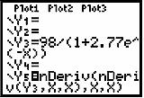
We are given , defining the percent of a population with a given characteristic with t = 0 corresponding to 1960 and t measured in decades.

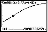
This function and its second derivative can be entered into the Y= screen as shown at below.

 

 

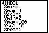
For this type of function, called a “logistic” model, we know that and that is always positive. We set a WINDOW for Y values from 0 to 100 and X values from 0 to 4. The graph of this function and the WINDOW are shown below.

 

 

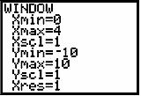
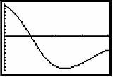
It appears that concavity changes from up to down somewhere near t = 1.

 

To see if the second derivative is 0 at a point near t = 1, we graph the second derivative which is Y5 in the first screen above. A choice of different values for Y makes the second derivative graph easier to see.

 

 

To find the zero of this second derivative, use and choose item number 2. You should get about 1.02 which represents the passage of one decade or the beginning of the year 1970 in our problem.