Word Lesson: Linear Regression
By D Saye
- know how to enter data for completing modeling problems
- know how to determine slopes of linear equations
- know how to calculate a linear equation that best fits a set of given data
- know how to solve literal equations
- recognize the science quantities associated with the slopes of special data sets
- know how to rearrange a literal equation so that an associated science formula can be used to discover the best interpretation of the slope of the trend line
- know how to write and solve an equation for a word problem
Examples of how linear regression is used in a science application can be seen in PhysicsLAB. Worksheets that accompany this lesson can be located under related documents, worksheets, Data Analysis #1-#8.
Let's look at an example of linear regression by examining the data in the following table to discover the relationship between temperatures measured in Celsius (Centigrade) and Fahrenheit. [Remember that lines are named using the convention y vs. x whereas data tables are constructed as x | y.]
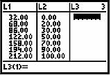
Fahrenheit degrees (ºF) | Celsius degrees (ºC) |
32 | 0 |
68 | 20 |
86 | 30 |
122 | 50 |
158 | 70 |
194 | 90 |
212 | 100 |
Based on this data:
- interpolate the equivalent temperature in degrees Celsius of our body temperature, 98.6 °F
- relate the linear equation of your model with its associated science formula to determine the "physical" meaning of the slope of this data's trend line
Step 1: First we will plot the data using a TI-83 graphing calculator. We will enter the data measured in degrees Fahrenheit in L1 and the temperatures measured in degrees Celsius in L2. Once the data is entered, your screen should look like the following:
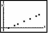
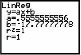
After entering the data into the calculator, graph the data. The Fahrenheit data, listed in L1, represents the x-axis, and the Celsius data, listed in L2, represents the y-axis. Your screen should look like the following:Step Two: Now we need to find a linear equation that models the data we have plotted. According to the calculator, our equation has the following properties:
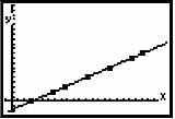
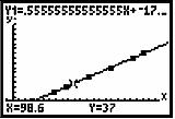
Our linear equation (rounded to thousandths) that best fits our data isStep Three: The graph of the function is shown below.
Based on the graph and the equation information listed above, our correlation coefficient (r) is equal to 1. That means that our data perfectly models a linear function.Step Four: Using the model from step two and the graph on our calculator from step three, we can trace along the graph and determine what temperature in degrees Celsius equals 98.6 °F, our body temperature.
This screen capture shows us that 98.6 °F (x-value) is equivalent to 37 °C (y-value).
Step Five: Consider our equation
. The accepted formula used to convert Fahrenheit degrees to Celsius degrees is typically written as
If we distribute the fraction
, we have
Expressed in this form we can clearly see that our model's equation is indeed the same equation conventionally used to convert temperatures between these two measuring scales. Since our line's slope [
] is a decimal, we know that the size of a "degree" on the two temperature scales is not the same; that is, these scales are not in a one-to-one correspondence -- 1 Celsius degree (Cº) does not equal 1 Fahrenheit degree (Fº).
Examining the slope in fraction form [
] we can clearly see that the relationship between the two scales is such that from a given point on the line, you move up five degrees on the Celsius scale and right nine degrees on the Fahrenheit scale to arrive at the next point on the line. Or equivalently, when the temperature changes 9 Fº it only changes 5 Cº.
Additionally, the y-intercept for our equation which tells us that when the temperature is 0 °F the temperature is -27.778 °C. The y-intercept is the point where the graph crosses the y-axis

Directions and/or Common Information:
No audio files were recorded for this set of examples.
Height (inches) | Weight (pounds) |
61 | 160 |
63 | 170 |
65 | 180 |
67 | 190 |
69 | 200 |
72 | 220 |
73 | 230 |
- extrapolate the weight of a 75-inch tall person who has a BMI = 30
- discover the "physical" meaning of the slope of the data's trend line
The table below lists distances in megaparsecs (3.09 x 10²² meters) and velocities in km/sec (1 x 10³ m/sec) of four galaxies moving rapidly away from the earth:
Galaxy | Distance (Mpc) | Velocity (km/sec) |
Virgo | 15 | 1600 |
Ursa Minor | 200 | 15,000 |
Corona Borealis | 290 | 24,000 |
Bootes | 520 | 40,000 |
- Use this data to extrapolate the velocity of Hydra, a galaxy located 776 megaparsecs from earth.
- Use the equation of your trend line and dimensional analysis to ascertain the "physical" meaning of its slope.
Directions and/or Common Information:
No audio files were recorded for this set of examples. Time (seconds) | Position (meters) |
1 | 9 |
2 | 12 |
4 | 17 |
6 | 21 |
8 | 26 |
- 33 meters
- 34 meters
- 35 meters
- 36 meters
Relative Humidity (%) | Apparent Temperature (ºF) |
0 | 64 |
10 | 65 |
20 | 67 |
30 | 68 |
40 | 70 |
50 | 71 |
60 | 72 |
70 | 73 |
80 | 74 |
90 | 75 |
100 | 76 |
- Approximately 76.6°F
- Approximately 77.7°F
- Approximately 78.4°F
- Approximately 65.7°F